Frequency Meter HP mod. 500B 1ª parte.

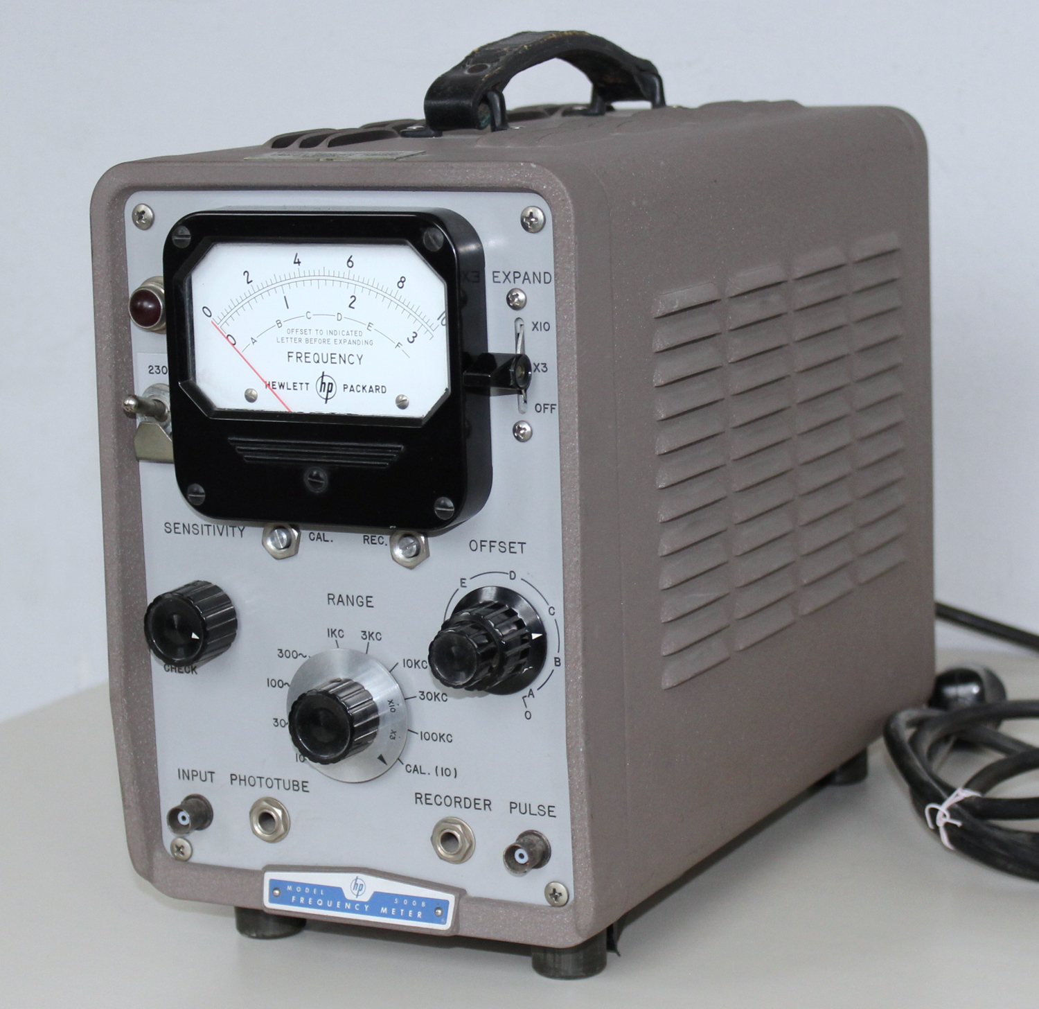
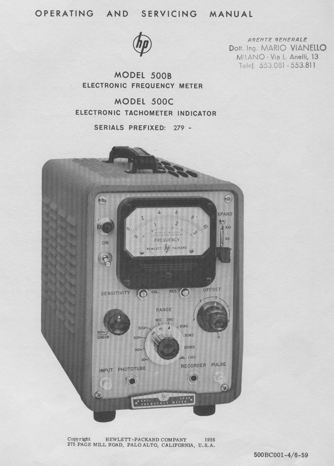
Frequency Meter HP mod. 500B. Prima parte.
Importato da Ing. Mario Vianello, Milano.
Nell’inventario D del 1956, in data 30 dicembre 1960, al n°  1858  si legge:  “Piaggio- Genova.  Frequenzimetro -hp-, mod. 500B, destinazione Elettronica”.
Nell’Estratto dell’Inventario ad uso della Sezione Elettronica, al n° 1858, in data giugno 1961, si legge: “Frequenzimetro portatile mod. 500B 3 Hz 100 Hz. Destinazione Laboratorio”.
Dono della Fondazione Carlo e Giuseppe Piaggio di Genova, come si legge nella targhetta visibile in una foto.
Un manuale di istruzioni si può trovare all’indirizzo:
http://hparchive.com/Manuals/HP-500B-C-Manual.pdf .

Noi riportiamo in due schede una parte del manuale del 1959 conservato presso la Sezione Elettronica. Abbiamo ritenuto opportuno omettere la sezione MAINTENANCE, per abbreviare il testo, ma inserendo alcune figure interessanti contenute in essa.§§§
«SECTION I GENERAL DESCRIPTION
1.1 GENERAL DESCRIPTION
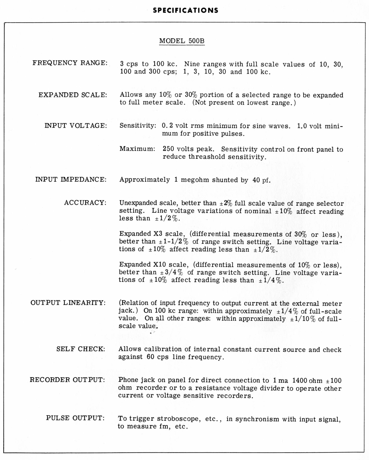
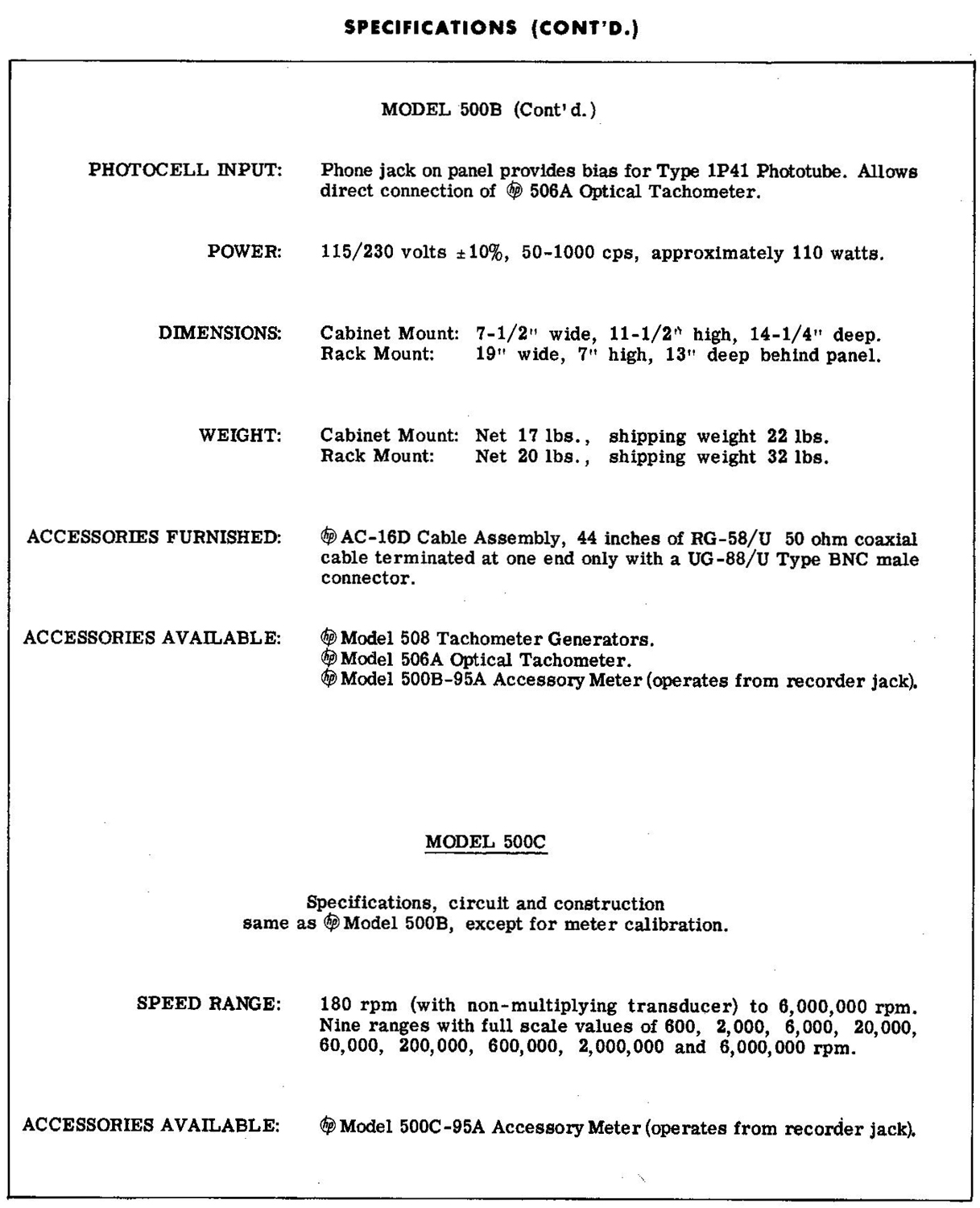
The Model 500B directly measures the frequency of an alternating voltage from 3 cps to 100 KC. It is suitable for laboratory measurement or production testing of audio and supersonic frequencies or for direct tachometry measurement with appropriate transducers, such as the -hp- 506A Optical Tachometer Pickup or the -hp- Model 508A/B Tachometer Generators. The indications of the meter are independent of input waveform, permitting the instrument to count sine-waves, square waves, or pulses and to indicate the average frequency of random events. A RECORDER  jack permits operation of a 1 ma recorder, such as the Esterline-Angus Automatic Recorder, for continuous frequency record. The impedance characteristics of this terminal may be adjusted to match any 1400 ohm (±100 ohm) 1 ma recorder to the 500B meter circuit. The RECORDER jack also may be employed to drive a remote indicating meter available from the Hewlett- Packard Company as an accessory. Besides indicating an applied frequency and providing a recorder output, however, the Model 500B is designed to be valuable in two other types of measurements. First, it is designed to be able to expand its scale readings by factors of 3 or 10 times, an arrangement that facilitates measurements of frequency changes such as might be caused by line voltage changes on frequency-generating circuits. Second, the instrument is designed to provide an output voltage which is proportional to the applied frequency. This signal from the PULSE terminal enables the instrument to be used as a wide band discriminator in applications where the measured signal contains very rapid frequency changes or frequency modulation. The discriminator voltage, when filtered, can be used to measure the amount of deviation in the signal as well as the rate and components of deviation. The Model 500C Electronic Tachometer Indicator is similar in circuitry to the 500B except for the meter calibration. The Model 500C is calibrated in terms of RPM with a counting range from 180 RPM to 6,000,000 RPM. In conjunction with the Hewlett-Packard Model 508B Tachometer Generator  the 500C will measure speeds from 15 to 40,000 RPM. When used with the Model 506A Optical due Tachometer Pickup the instrument is capable  of measuring very high speeds of moving parts which have small energy, or which for mechanical  reasons  cannot tolerate mechanical loading.
1-2 DAMAGE IN TRANSIT
Instructions and information concerning shipping  damage are contained in the WARRANTY section on the last page of this manual.
1-3 POWER TRANSFORMER CONVERSION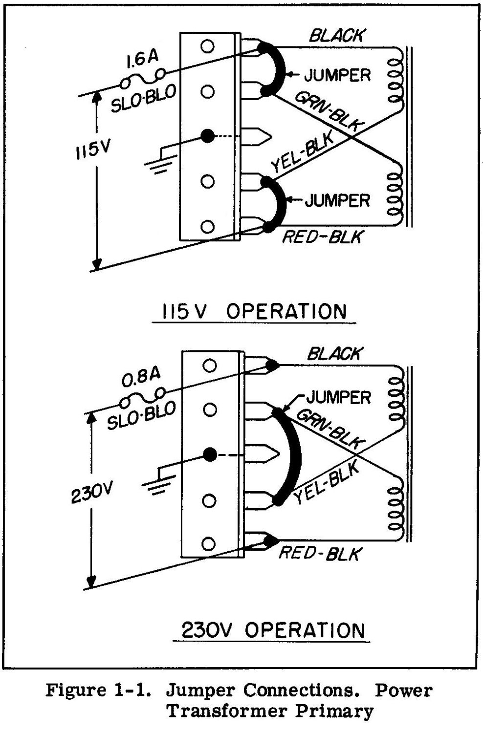The Model 500B may be easily converted  to operate from a 230 volt line source by removing the bare wire jumpers from the terminal strip, located beneath the power transformer, and inserting a new jumper as shown in Figure 1-2.

As shown in the schematic diagram the 230 V connection changes the primary winding arrangement from parallel (115V) to series (230 V). After converting the instrument to 230 volt  operation, change the line fuse, as shown, to 0.8 amperes, slo-blo.
1-4 RPM MEASUREMENT WITH TACHOMETER GENERATORS
The Model 500B measures RPM and RPS by measuring an electrical frequency that is proportional to the speed of a rotating shaft. Generation of this frequency may be accomplished by several types of transducers which allow considerable latitude in measurement technique. A simple and direct way to measure RPM is through the use of a tachometer generator that produces a frequency that is proportional to the speed of its own shaft. The -hp- Models 508A and 508B are examples of this type of transducer, and are recommended  for use with the Model 500B. Both are of the variable reluctance type and have no brushes or slip rings to cause noise or random irregularities that result in inaccurate readings. Other types of generators may be used if they have an output frequency proportional to their shaft speeds and are free of electrical noise and transients.
(Limiting case: S/N = 1.) To assure accurate counts, the use of an oscilloscope to check the signal from other types of tachometer generators is recommended.
1-5 ACCESSORY TACHOMETER GENERATORS
The -hp- Models 508A and 508B are compact low-torque tachometer generators. The Model 508A produces 60 ∼ for each revolution of its drive shaft, while the Model 508B produces 100 ∼ for each shaft revolution. When using the 508A the Model 500B indicates shaft speed directly in RPM. When using the 508B, the displayed answer is divided by 100 to obtain revolutions/sec. When using the 508B, the Model 500C indicates RPM directly when divided by 100. The useful shaft speed range for Model 508A Tachometer Generator is from approximately 15 RPM to 40,000 RPM. Consequently, this tachometer generator is entirely suitable for all shaft speeds normally encountered. The output voltage from these transducers increases almost linearly from 15 RPM to 5000 RPM from a minimum of about 0.1 volt RMS to a maximum of almost 10 volts. At shaft speeds above 5000 RPM, the output voltage decreases gradually to a value of about 1 volt at 40,000 RPM. The linear relationship between out-put voltage and shaft RPM to about 5000 RPM provides  a very useful auxiliary function for the tachometer  generator. The speed-voltage relationship makes it possible to present on an oscilloscope screen a curve describing the instantaneous rate of rotation of a shaft as a function of time. This allows analysis of the instantaneous effect on rotating equipment from the action of clutches, brakes, or other mechanical components. For this application, connect the output of the tachometer generator to the vertical deflection  plates of an oscilloscope. Since the data presented on the oscilloscope screen is usually nonrepetitive in nature, a photographic record is normally made. Torsional vibration, harmonic-ringing and the action of intermittent motions are shown as a function of time by variations in the height of the oscilloscope trace.
1-6 PHOTOELECTRIC TACHOMETRY
Photoelectric tachometry pickups have three particular advantages: they are effective over a wide range of speeds; they are easily adaptable to a wide range of situations; they do not load a system  under measurement. The Model 500B is designed for use with photoelectric transducers and a special connector (PHOTOTUBE), located on the front panel of the instrument, supplies the necessary  bias voltage to a photocell of type 1P41 or equal. This jack serves also as the signal input jack for this application. The Model 506A Tachometer provides for counting speeds or revolutions over a wide range from about 300 RPM (5 RPS) to 300,000 RPM (5,000 RPS). The light source in the Model 506A Tachometer Pickup illuminates a moving part which is prepared with alternate reflecting and absorbing surfaces. The interrupted reflected light is picked up by the phototube and the electrical impulses generated are transmitted to the 500B. This system is positive in action and the danger of fractional or multiple errors inherent in other measuring methods is eliminated. For best results, the size of the reflecting and absorbing surfaces should be approximately 3/4 in. square. This means that the shaft whose speed is to be measured should have a diameter of at least 1/2 inch. The speeds of smaller diameter shafts may be measured by installing a sleeve of larger diameter, or by providing a rotating, reflecting, and absorbing surface at right angles to the plane of the shaft. Surfaces such as these are also used for increasing resolution in measurement of low RPM where the multiple absorbing and reflecting surfaces provide a large number of impulses per revolution. When this is done, a division factor is applied to the reading obtained on the Model 500B. The -hp- Model 506A consists of a pair of shielded tubes, one of which contains an incandescent light source, while the other houses a Type 1P41 Phototube. These are equipped with condensing lenses and are so oriented that proper focus is obtained at a distance between 3 and 6 inches from the reflecting surface. The light source and phototube assembly is mounted on an adjustable stand for optimum positioning of both light source and phototube. The base of this stand contains a transformer which provides the proper voltage for operating the incandescent lamp. The phototube requires a bias voltage from +70 to +90 volts. This voltage is automatically supplied by the PHOTOTUBE jack on the -hp- Model 500B.

SECTION II OPERATING INSTRUCTIONS

SECTION  IIA
2A-1 GENERAL
The operating instructions for the 500B and the 500C are given in two separate sections. The 500B is covered in Section IIB and the 500C is covered in Section IIC. The instruments are identical electrically. The only difference is the meter face calibration and the range selector markings. The paragraphs in the 500B which cover accuracy of measurements, random counting procedure, recorder operation, and pulse applications, are not repeated in Section IIC, although they apply equally well to the 500C.SECTION  llB
500B OPERATING INSTRUCTIONS
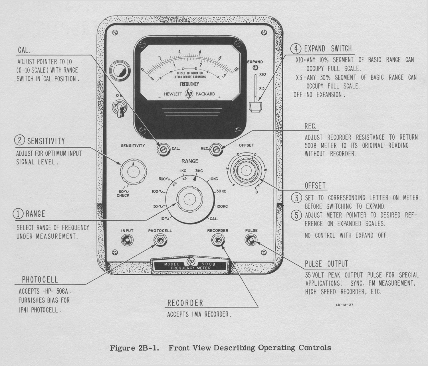
2B-1 CONTROLS AND TERMINALS
SENSITIVITY
This control, normally in the maximum position, is used to decrease the sensitivity of the input amplifier to eliminate errors resulting from spurious modulation of the desired signal.
60 ∼  CHECK
This switch position on the SENSITIVITY control places the line frequency into the input circuit. With the RANGE switch in the appropriate position (usually 100∼) and the EXPAND switch OFF, the meter should indicate the frequency of the line voltage.
RANGE
This rotary switch selects the desired frequency range.
CAL
The CAL position of the RANGE switch checks satisfactory calibration of the constant current source in the circuit by indicating full scale on the 0-10 scale. In this position, input signals have no effect upon the meter.
CAL ADJUST
This screwdriver adjustment is used to calibrate the constant current source. See paragraph 2-9.
EXPAND
Expands any 10 percent (X10) or any 30 percent (X3) of the basic range in use to full scale. Use of the expanded scale is discussed in paragraph 2B-3.
INPUT
This BNC connector accepts any unknown signal from 0.2 to 150 volts rms.
PULSE
This BNC connector is an output terminal providing 35 volt peak pulse out for special applications (see paragraphs 2B-12, 2B-13).
PHOTOTUBE
This phone-type jack furnishes bias for a 1P41 phototube permitting the direct connection of the -hp- Model 506A Optical Tachometer.
RECORDER
This phone-type jack is provided for connecting a 1 ma recorder to the instrument.
REC  ADJ
This screwdriver-operated potentiometer adjusts the effective resistance of a recorder to match the instrument. The adjustment procedure is described in paragraph 2-B-9.
2B-2 OPERATING PROCEDURE, COUNTING
a. Allow a. period of five minutes for the instrument to reach a stable operating temperature after turning ON.
b. Turn the SENSITIVITY control to the maximum clockwise position. Place the EXPAND switch to OFF.
c. Set the RANGE switch to the 100 KC position.
d. Place signal under test across the INPUT connector.
e. Step the RANGE switch down from the 100 KC position as necessary until the meter pointer rests in the top 2/3 of the meter scale. Decrease the SENSITIVITY control and watch for a change in the reading. The reading should remain constant over a plateau of control to assure you that noise modulation is not being measured as part of the signal under test.
It is necessary with unknown input frequencies to start the RANGE switch at 100 KC and step down, because inputs in excess of values on RANGE switch can overdrive the instrument to display erroneous readings, i.e.: 2 KC will be erroneously displayed on the 1 KC range, but not on3 KC range and above.
2B-3 EXPANDED SCALE. GENERAL
The expanded scale feature allows increased accuracy in the measurement of changes in frequency by magnifying pointer action. The pointer action is magnified by expanding to full scale a 30 percent segment (X3 setting of the EXPAND switch) or a 10 percent segment (X10 setting of the EXPAND switch) of the range selected by the RANGE switch. The particular expanded segment represented  by the meter scale is determined by the concentric OFFSET controls, which move the segment between zero and full scale of the basic range. Since the segment selection is arbitrary and the meter pointer always indicates the value of the input signal, the meter pointer will be on scale only if the selected segment includes the frequency of the input signal. The number of cycles in the segment is indicated by the X3 or X10 on the skirt of the RANGE switch (see Figure 2B-2).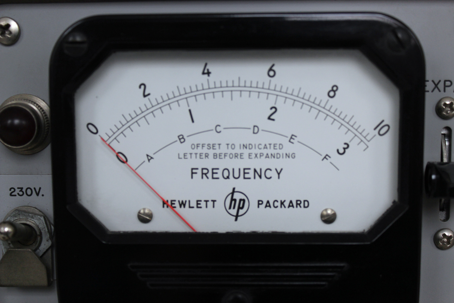A letter system helps find the segment which includes the input signal; the letters are marked both on the meter face and around the OFFSET controls. When an unexpanded measurement is made, the meter pointer indicates a point on the letter system as well as the value of the input signal, and the coarse OFFSET control should be set near that point of the letter system before the EXPAND switch is actuated. When the EXPAND switch is actuated, the meter pointer will be on scale or not far off scale, and slight adjustment of the OFFSET controls will set the meter pointer to the desired place on the scale. Presetting the OFFSET controls makes it easier to find the segment which includes the input signal and prevents the meter pointer from violently pinning off scale when an expanded scale is selected.
Four things must be remembered when the expanded scales are used:
1.The setting of the OFFSET controls is arbitrary! Any segment may be chosen. However, only segments which include the input signal are useful.
2.The letter system is a guide to help find the segment which includes the input signal. It is not exact.
3.The numbers on the meter scales do not indicate specific frequencies because the segment can be set anywhere along the basic range. However, if the selected segment includes the input signal, the pointer indicates the relative positionof the input signal within the segment. If the segment does not include the input signal, thepointer will be off scale.
4.Calibration of the meter scales is determined by the position of the pointer, the basic range selected, and the degree of expansion. For example, if the 1 KC range is expanded X3, the 0-3 scale becomes a 300 cps segment of the 1 KC range. If the pointer is placed over the 2.8 marker by the OFFSET controls, and it subsequently moves to the 1.3 marker, a 150 cps decrease in the input signal is indicated.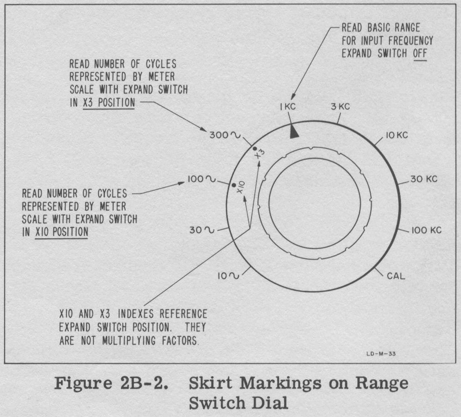The following paragraph describes the use of the
expanded scale by following through a differential
measurement example.
2B-4 EXAMPLE PROCEDURE
a.Connect the Model 500B to proper source; turn on the power switch and allow five minutes for the instrument to reach a stable operating temperature.
b.Make an unexpanded measurement of the input signal as described in paragraph 2B-2. Assume that the measurement is 700 cps on the 1 KC range, and that ±100 cps variation is to be observed. Note that the meter pointer rests between D and E on the letter system. See Figure 2B-3.
c.Adjust coarse OFFSET control to the corresponding point between D and E on the letter system around the control.
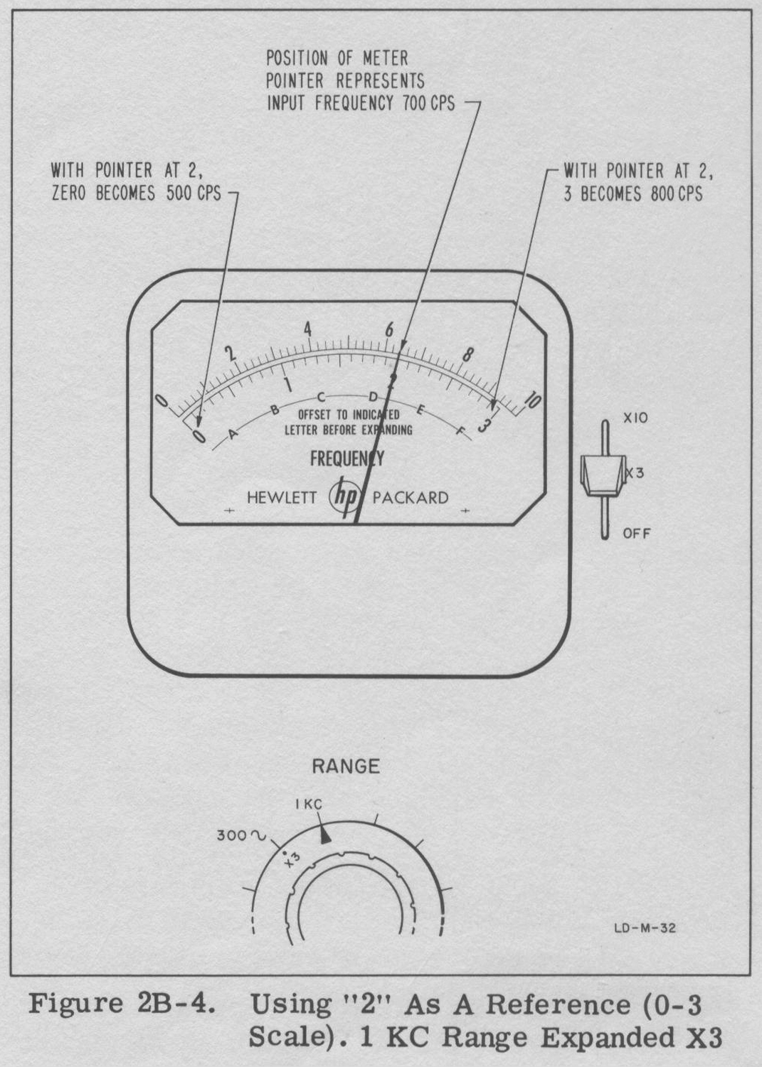
d.Place EXPAND switch to X3 position. With the EXPAND switch in the X3 position, the 0-3 scale is a 300 cps segment of the 1 KC range.
e.Refine OFFSET adjustment to place pointer at the desired reference. The meter pointer can be placed anywhere on the expanded scale, but to observe the ±100 cps variation, the pointer must be at least 100 cps from either end of the scale.
Suppose the pointer is placed at “2” on the 0-3 scale. Figure 2B-4 illustrates the resulting calibration of the meter scale.
If the pointer had been placed at “0”, then “0” would have become 700 cp, and the meter scale would have displayed a 300 cps segment from 700 cps to 1,000 cps with the 1,000 cps point at “3”. In this case, only the +100 cps variation could be observed.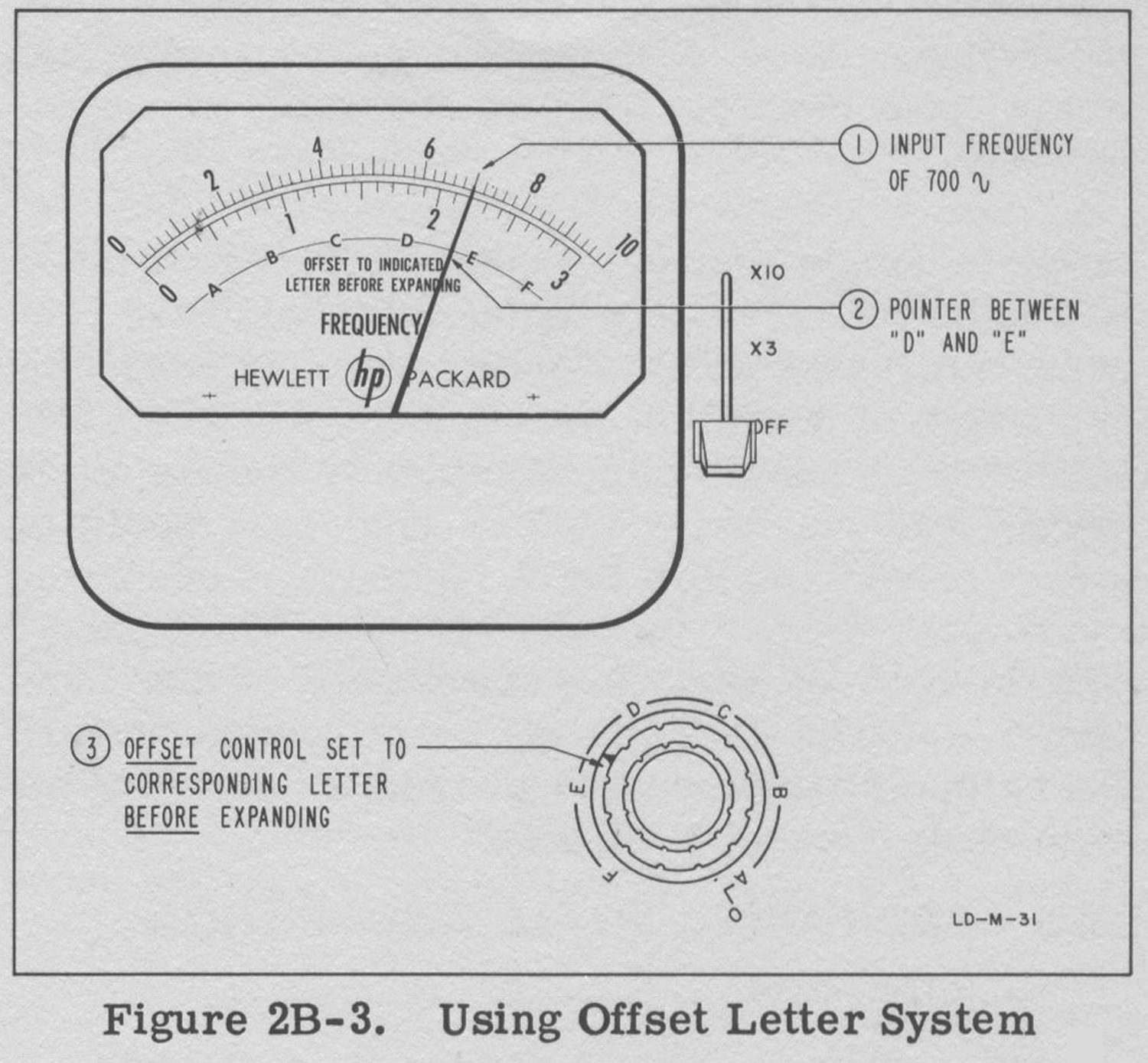2B-4A  EXAMPLE SUMMARY
Control of the meter pointer allows an arbitrary calibration of an expanded scale within a small segment of the basic range. This control establishes a reference point suitable to a particular differential or comparative measurement. In the example developed above, the expanded segment contained 300 cps displayed full scale with an input frequency of 700 cps. Greater pointer, excursion occurs per cycle of variation than would occur using the unexpanded 1 KC scale. The greater pointer excursion allows more sensitive observation of fluctuations, variations, and drift in the input signal. It displays these changes more accurately than would have been possible on the 1 KC range unexpanded. In the example above, suppose a ± 50 cps variation was to be observed. X10 expansion could have been used to present an even greater pointer excursion per cycle of variation than that for X3. In the X10 case, the segment would contain only 100 cps (0- 10 scale), and the meter pointer (700 cps) would be placed at “5” to allow the variation to be observed. The amount of variation anticipated on the input signal governs the amount of expansion chosen. Paragraph 2B-6 discusses instrument accuracy for each measurement condition.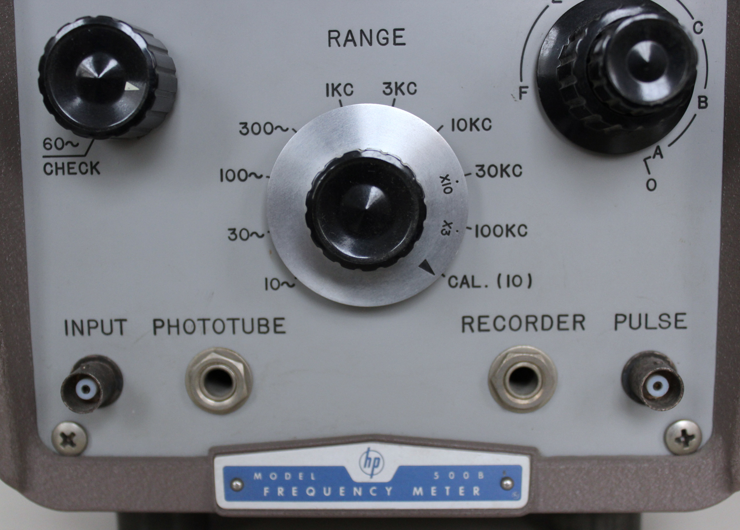2B-5 ADDITIONAL SCALE CALIBRATION METHODS
In the example of paragraph 2B-4 the expanded scale was calibrated with the input frequency for differential measurement. The accuracy of such a calibration is limited by the basic accuracy of the unexpanded scale used for the initial measurement, i.e. ±2 percent full scale, but the measurement accuracy of change in frequency is improved (see paragraph 2B-6). Another method of calibration, useful in random counting, for example (paragraph 2B-7), consists of placing both OFFSET controls fully clockwise. This action calibrates the expanded scale “0” as zero cycles, and calibrates full scale to the magnitude of the segment. For example, the 10 KC range expanded X10 with the OFFSET controls fully clockwise would calibrate the 0 to 10 meter scale from 0 to 1 KC. Calibration of expanded scale with a known frequency, such as a standard or calibrated oscillator,  can also be accomplished to improve the accuracy of expanded scale calibration. In this method an accurate frequency, close to the unknown in magnitude, would drive the instrument to establish a convenient calibration on the expanded scale. This signal would be removed and the unknown signal would be measured on the instrument without changing the OFFSET control.
2B-6 ACCURACY OF MEASUREMENTS
The basic accuracy of measurement on an unexpanded range of the Model 500B is better than ±2% of full scale value for any range in use. In this discussion the term full-scale, whether or not the scale is expanded, always relates to the frequency value shown under the arrow marker on the RANGE switch dial skirt. This accuracy applies only to single frequency measurement. When differential measurements are made two readings are implicit in the process, and the double liability of error doubles the possible error. As shown in Table 2B-1, the unexpanded scale accuracy is ±2% full scale for single frequency measurement and is 13.5% full scale for differential measurement. In examining the various sources for error in the first two columns of the table, it is seen that all errors double in differential measurement, except the circuit calibration error which is linear, always in the same direction, and constant for single or differential frequency measurement. Moving to the third column, X3, it is seen that the sources for differentia1 error are divided by three-except  the phantastron timing error which remains constant. This error is not reduced upon expanding  because it arises in the phantastron circuit with line variation. The timing error varies the length of the constant current pulses to produce an erroneous meter indication which is expanded along with the scale expansion so that it remains constant percentage when related to the full-scale range value. All other errors are related to “pin to pin” meter behavior and remain constant in percentage when related to the number of scale divisions on the meter. The effect is to reduce the percentage full-scale  error when the scale divisions are related back to the unexpanded full-scale value. For example, consider meter tracking error on the 100 KC range as ±1%. This is ±1/2 scale division or ±100 cps. Expanding the 100 KC range to X10, ±1% then becomes ±1/2 scale division or ±100 cps. Relating this 100 cp back to  full-scale value, 100 KC, meter tracking error becomes ±0.1%: doubled for differential error it becomes ±0.2%. Thus, expanded scale error is determined in all cases, except phantastron timing, by dividing the basic range error by the factor of expansion, and then doubling this quantity to obtain total differential error. The last three columns of Table 2B-1 show maximum possible errors when differential measurements are made with constant line voltage. In these cases the errors arising from line voltage variation become zero. It should be noted that the line variation (assuming a 115 V line) described for the first four columns of the table constitutes a 30-volt fluctuation from 130 volts to 100 volts or from 100 volts to 130 volts, between readings. Most measurement conditions will be better than this with a substantial improvement in the accuracy of the Model 500B.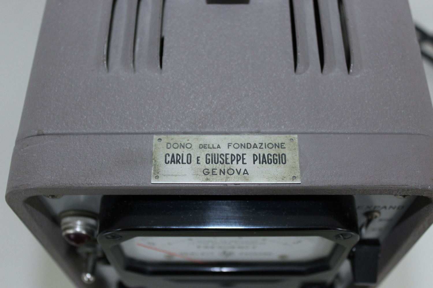2B-7 RANDOM COUNTING, GENERAL
During random counting operation several instrument considerations should be kept in mind by the operator: (1) the time constant of the meter, (2) the basic full-scale accuracy of the meter, and (3) a predictable error arising from the nature of the internal pulse forming circuit. These considerations will be discussed in the following paragraphs.
2B-7A METER TIME CONSTANT
Since the random count is averaged over the time constant of the meter, in some applications of measurement the meter pointer may exhibit a tendency to vibrate or oscillate about the average reading. In some cases this vibration may become severe enough to inhibit readings. If this situation occurs it is recommended that a capacitor be placed in the meter circuit to increase its time constant. The capacitor should be placed from the plus (+) side of the meter to ground. The capacitance used will depend upon the particular application,  but 500 μf has been found sufficient to damp the vibration in most cases. If desired, the Hewlett-Packard Accessory Meter (described in Specifications) could be modified by placing 500 μf directly across its terminals and used for random counting operation.
2B-7B BASIC ACCURACY
The basic accuracy of the Model 500B/C is 12% full-scale division. The effect of this error is minimized for the frequency of interest as the pointer approaches a full-scale indication. In measurement operation it is desirable to maintain the pointer as close to a full-scale indication as practicable.
2B-7C PREDICTABLE ERROR
In random counting the possibility of missing an input pulse while the circuit is developing a current pulse from the previous signal constitutes a predictable error. Since the constant current pulse, developed internally, occupies approximately 60 percent of the period time for any given basic RANGE position, unexpanded, a correction factor can be formulated to correct readings.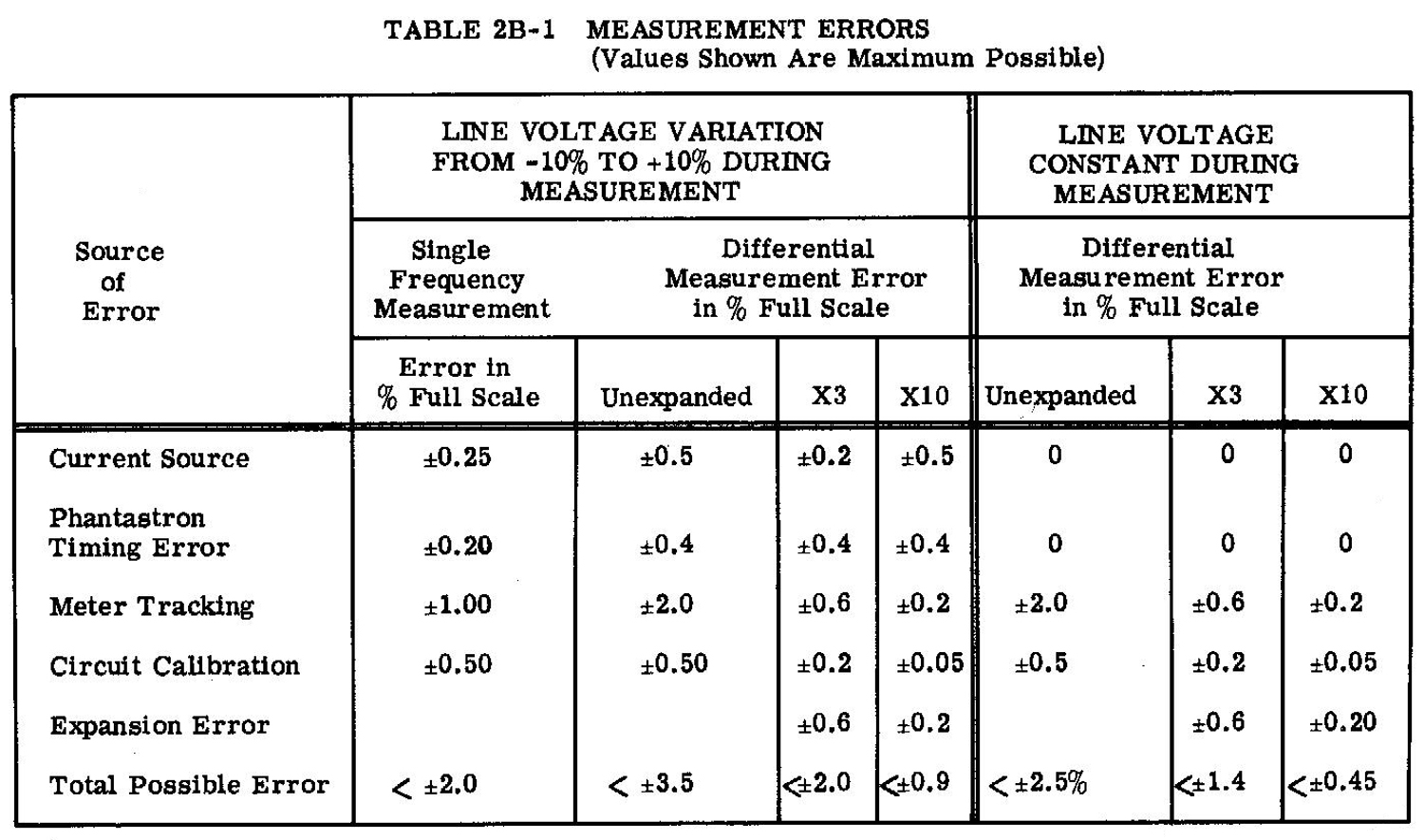If F = random average frequency,
and f_i = indicated frequency,
and  f_s = frequency represented by full scale in use,
and d = width of current pulse × number pulses,
then d = .60/fs(fi).
The time available for counting an input pulse is given by the expression:
Time avail. ≅ 1-d or 1 – .60 f_i / f_s
The random average frequency with no expansion is:

 F ≅  f_i /[1- (.6 fi/fs)].  (1)    

With X10 expansion:  

F  ≅  f_i / [1- (.06 fi/fs)]   (2). 

With X3 expansion:

F ≅ f_i / [1- (.2 fi/fs)]   (3).  ».
§§§
Il testo prosegue nella seconda parte; per consultarla scrivere “500B” su Cerca.
Foto di Claudio Profumieri, elaborazioni e ricerche di Fabio Panfili.
Per ingrandire le immagini cliccare su di esse col tasto destro del mouse e scegliere tra le opzioni.