Frequency Meter HP mod. 500B. Seconda parte.
Nell’inventario D del 1956, in data 30 dicembre 1960, al n° 1858 si legge: “Piaggio- Genova. Frequenzimetro -hp-, mod. 500B, destinazione Elettronica.”
Nell’Estratto dell’Inventario ad uso della Sezione Elettronica, al n° 1858, in data giugno 1961, si legge: “Frequenzimetro portatile mod. 500B 3 Hz 100 Hz. Destinazione Laboratorio”.
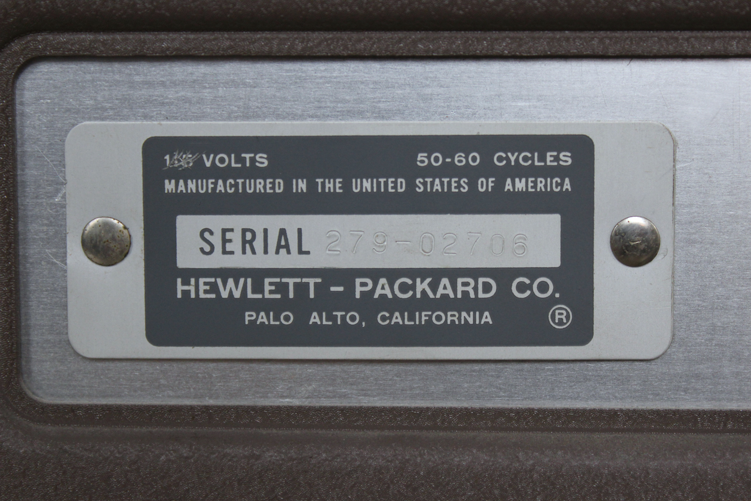
Dono della Fondazione Carlo e Giuseppe Piaggio di Genova, come si legge in una targhetta qui visibile in una foto.
Un manuale di istruzioni si può trovare all’indirizzo:
http://hparchive.com/Manuals/HP-500B-C-Manual.pdf
Il testo prosegue dalla prima parte.
§§§
«2B-8 RANDOM COUNTING PROCEDURE
a.Place controls in the following positions:
RANGE – 100 KC
EXPAND – X10
OFFSET – both controls to zero, full clockwise.
Under these conditions the zero position of the OFFSET control calibrates zero on the meter (0-10 scale) so that an absolute reading may be obtained on the expanded scale from zero to 10 KC. The 10 KC range is not used because, as explained in paragraph 2B-7C, 60 percent of the period time of a basic range frequency is used to develop the current pulse and is not available for counting. Less time is used developing the shorter current pulses for the 100 KC range than is used for those developed on the 10 KC range. This means that by expanding you achieve a reading which is closer to the actual random count, since the probable counts missed during the development of the constant current pulses through the meter will be fewer. Thus the correction which is applied as the “predictable error” will be smaller in magnitude. However, unexpanded ranges may be used. The disadvantage is that the readings will be further from the actual count, and the “predictable error” correction will be correspondingly larger.
b.Place the input signal across the INPUT terminals.
c.Note the reading on the meter and step down the RANGE switch as necessary to obtain a satisfactory meter reading. As the RANGE switch is stepped down, is in equations (1), (2), and (3) is reduced, and the “predictable error” correction increases. However, the basic meter accuracy -an unpredictable quantity – improves because the meter pointer indicates further upscale as the RANGE switch is stepped down.
d.When the indicated reading has been obtained apply the applicable correction factor from equation (2) for X10 expansion, or equation (3) for X3 expansion.
———EXAMPLE ———-
With the instrument set up as described in steps a. and b. above, a measurement is taken and the RANGE switch is stepped down to the 10 KC position. This action places the X10 marking in the RANGE switch dial skirt at 1 KC. The meter reads 4.5. Therefore, it represents an uncorrected average count of 450 cps. Applying equation (2) for a random average count we have:
F = fi/[1 —.06fi/fs]
= (450)/{[1-.06(450)]/1000}
= 450/ .973
= 462 cps(±1 scale division)
————————————–
2B-9 OPERATING CALIBRATION AND CHECK
Two performance checks are available for the operator in checking the accuracy of the instrument during operation. Perform CAL check first. If two checks cannot be made to agree, see paragraph 4- 10.
CALIBRATION (CAL)
This check permits amplitude of the pulse from the constant current source in the meter to be calibrated. The procedure is as follows:
a.Turn on the instrument and permit it to reach a stable operating temperature.
b.Switch the RANGE control to CAL.
c.Adjust the CAL ADJ potentiometer with a screw-driver so that the meter indicates full scale (10) on the 0- 10 scale.
60 ∼ CHECK
This check places 6.3V at power line frequency across the input circuit of the meter.
To perform the check, switch the SENSITIVITY control to the 60 ∼ CHECK position and place the RANGE switch to a position which includes the known frequency of the power line. The line frequency should be indicated on the meter.
2B-10 RECORDER OPERATION
The Model 500B will drive any 1 ma, 1400 ohm (±100 ohm) recorder. When a recorder is used with the instrument the REC ADJ compensating resistor in the instrument must be adjusted to match the resistance of the recorder to that of the meter circuit. The adjustment procedure is as follows:
a.Allow the 500B to reach a stable operating temperature, and place the SENSITIVITY control in the 60 ∼ CHECK position. Adjust the RANGE switch to
include the line frequency, and note reading on meter.
b.Plug recorder into the RECORDER jack and adjust the REC control on the front panel so that the meter indication on the Model 500B is identical to the reading obtained in step a., above.
c.Use mechanical adjustment on recorder to obtain reading, above, on recorder scale.
When the recorder is removed from the circuit the REC adjusting potentiometer is removed from the meter circuit so that the accuracy of the 500B is unimpaired. The external recorder is placed in series with the meter in the 500B, and it tracks with the meter in the 500B. Thus, expanding a scale on the 500B simultaneously expands the recorder scale.
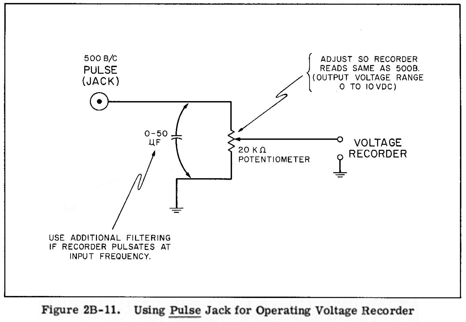
2B-11 RECORDER JACK RESPONSE
The current at the 500B recorder jack is proportional to the frequency of the input signal. This current is derived from a succession of pulses
and is averaged by means of a simple R-C integrating circuit. On low frequency ranges, it is necessary that the integrating time constant be long enough to prevent excessive flutter of the meter or recorder. This integrating also slows down the response of the meter and recorder current to sudden changes in frequency on the low ranges.
For example, on the 10 cps range, the integrating time constant is 200 milliseconds. Thus, when the frequency of the input signal changes suddenly, there will be an observable lag in the response of the meter or recorder. In fact, after 200 milliseconds, the meter needle will have moved only 63 percent of the distance between the old and new readings. It will move 90 percent of the distance in about one and a quarter seconds. If the input frequency varies about its average value in a sinusoidal manner, the output current will also vary sinusoidally about its average value. The amplitude of this current variation will also be reduced by the integrating circuit. An integrating time constant of 200 milliseconds corresponds to a high frequency cut-off of 0.8 cycles-per-second. Thus if the input frequency is varying at a 0.8 cps rate, the resulting current variation will be attenuated by 3 db, and its phase will lag that of the frequency variation by 45°.
The table below shows the integrating time constants (T) and cutoff frequency (Fco) for various range settings and expansion conditions on the 500B. The effective rise time (0-90%) of the out-put current is equal to 2.3T.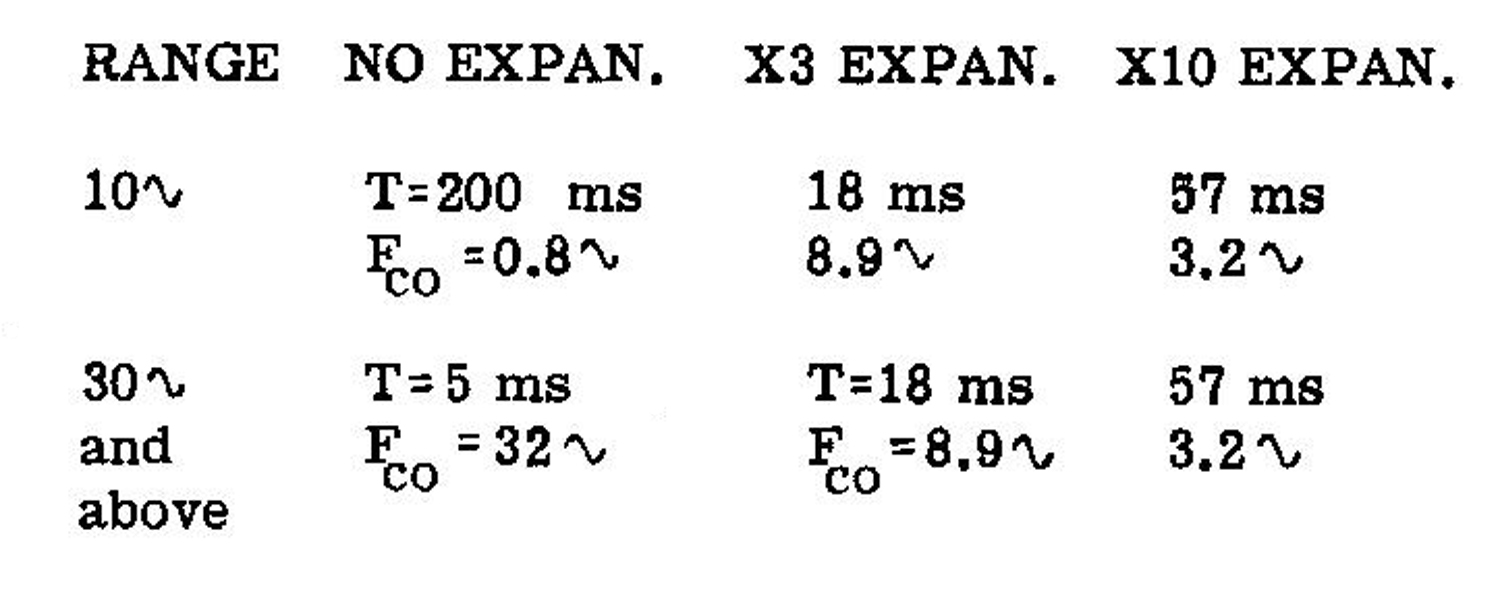 2B-12 PULSE OUTPUT RESPONSE
The voltage from the PULSE output terminal can be used to drive a recorder at higher speeds than are obtainable using the meter current from the recorder jack. It can be used to drive a stroboscope or sync an oscilloscope. The PULSE terminal produces voltage pulses which are identical in shape to the current pulses used in the meter circuit. Since this output signal is direct coupled, it contains a dc component which is proportional to frequency. However, the fact that it consists of unfiltered pulses allows the user to filter the response as desired.
The PULSE output consists of one negative voltage pulse for every cycle of the input signal. These pulses have an amplitude of -35 volts peak and a constant width such that a full scale meter reading (unexpanded) produces an average voltage of -20 volts. The pulse width is about 6/10 of the period corresponding to a full scale frequency.
For example, on the 100 KC range every input cycle produces an output pulse about 6 microseconds wide and -35 volts high. This pulse is presented at a resistive output impedance of about 23,000 Ω. If the terminal is shunted by a capacity of .01 microfarads, a filter time constant of RC = 200 microseconds will result. This will produce a maximum peak-to-peak ripple of (6/200) × 35 volts = 1.05 volts, which is 5.25 percent of full scale. This maximum ripple only occurs at frequencies which correspond to readings at the very low end of the meter scale. The ripple will decrease to about 4/10 of this maximum for full scale readings. Thus, at 100 KC the peak-to-peak ripple would be about 2 percent of full scale if a .01 mid shunt condenser was used to produce a filter time constant of 200 microseconds. This corresponds to a high frequency cut-off of 1/2 RC = 800 cps.
This frequency limit can be extended by using a shorter time constant if more ripple can be tolerated. Although the single shunt condenser is the simplest filter for this application, much better results can be obtained with a multi-section filter properly designed to reject signals at the input frequency and higher.
The particular filter to be used depends upon the application. For example, if it is desired to measure the deviation of a 60 KC signal which is being frequency modulated at 1000 cps, a 1000 cps bandpass filter can be used to select to 1000 cps component from the output terminal and present it to an ac voltmeter which can be accurately calibrated in deviation (20 volts = 100 KC on top range.)
2B-13 PULSE OUTPUT APPLICATIONS
How the PULSE output of the frequency meter proves valuable in measurements can be described by assuming that a frequency of 50 KC is to he measured. Assume further that this frequency contains a ±5 KC frequency modulation swing at a 1 KC rate and that it is desired to investigate this f-m.
When the frequency-modulated waveform is applied to the frequency meter, the panel meter will indicate the average frequency of 50 KC. For each cycle of the applied frequency, a voltage pulse will be available from the PULSE terminal, as shown in Figure 2B-5. Since the amplitude and width of these pulses are constant, and since the pulses are negative from ground, their short-time average value will vary in exact accordance with the frequency modulation they contain. The original modulating waveform can therefore be recovered if the pulses are averaged with a suitable low-pass filter.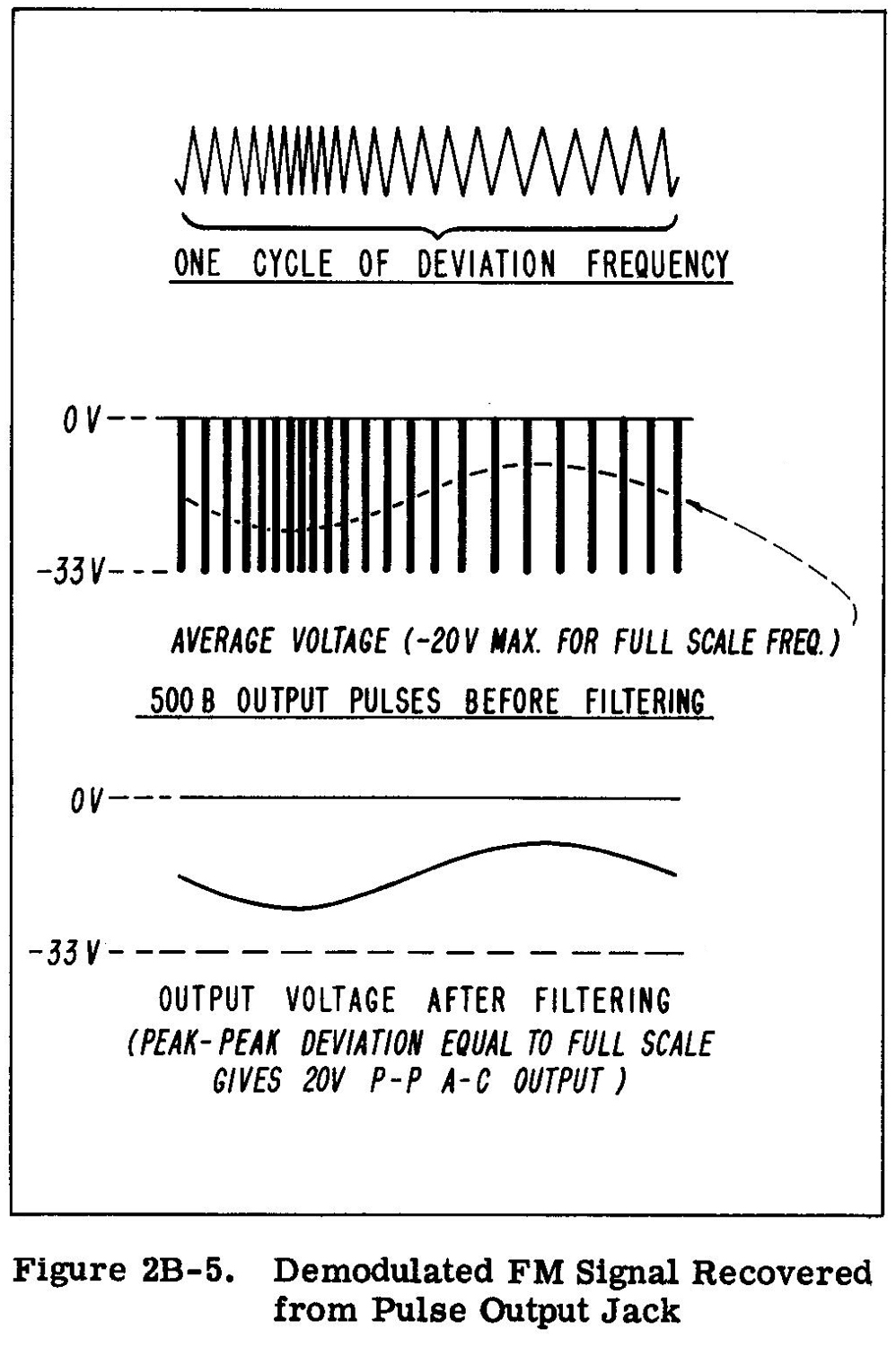 Not only can the waveform be recovered, but the amount of deviation in the signal can readily be measured, because the peak-to-peak amplitude of the variations in the short-time average level will be exactly proportional to the deviation. Since the amplitude and width of the output pulses is such as to give a d-c output level of -20 volts for a full-scale reading on the meter, the applied frequency of 50 KC in this example would cause a half-scale reading on the 100 KC range and therefore an average d-c output of -10 volts or -0.2 volt d-c/KC. By now measuring the peak-to-peak amplitude of the varying component of the d-c output with an oscilloscope or a-c voltmeter, the ± 5 KC deviation in the signal will be found to cause a measured value of 2 volts peak-to-peak.
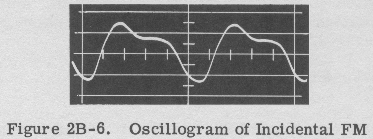
 In practice, these voltages will all be affected by the impedance of the filter used. The voltage per cycle or per kilocycle out of the filter can easily be determined by dividing the measured d-c voltage out of the filter by the reading on the frequency meter. A filter suitable for the example above and most applications is shown in Figure 2B-5A. The output of this filter is down 3 db at 15 KC, 5 dB at 18 KC, 10 db at 20 KC, and more than 55 dB at 23 KC and above. The filter need not always be as elaborate as the one shown in Figure 2B-5A; in some cases a single shunting capacitor will do. The cut-off frequency of the filter may be adjusted to any frequency in the audio range, but it must be higher than the modulation frequency and lower than the lowest frequency of the modulated signal. In order to obtain a fair approximation of the modulation signal from the output of the filter, there should be at least ten pulses into the filter for each cycle of the modulation frequency out of the filter. Thus, the average frequency of the modulated signal applied to the 500B should be at least ten times the modulation frequency. For example, if modulation components up to 5 KC are to be measured, the average frequency supplied to the input of the 500B should be not less than 50 KC. Figure 2B-6 is an oscillogram of a demodulated f-m signal recovered by using the PULSE output of the frequency meter in the method described in paragraph 2B-13. The waveform itself is theincidental f-m modulated into a klystron oscillator from the heater circuit.
2B-14 MEASURING KLYSTRON INCIDENTAL FM
Incidental f-m in the klystron output is translated to the range of the frequency meter by applying the klystron output to an -hp- 540A Transfer Oscillator.1 The Transfer Oscillator is tuned to produce a difference frequency of 70 KC which also contains the incidental f-m. Test arrangement shown in Figure 2B-7.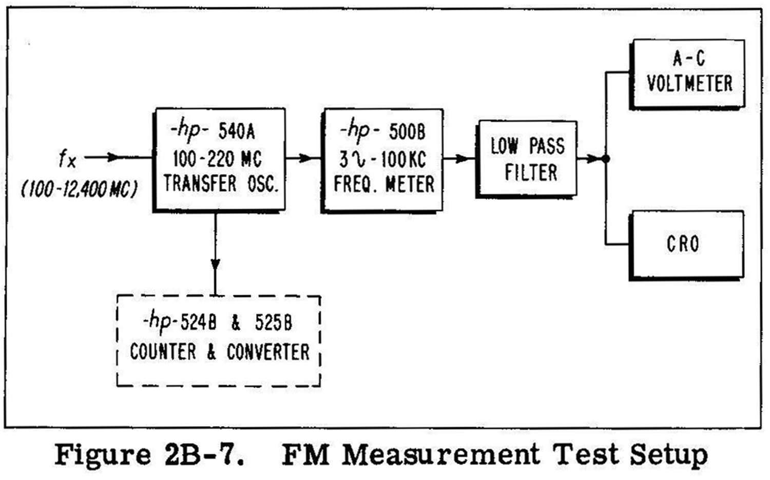 The amplitude of the deviation is measured by adjusting the oscilloscope gain to calibrate the scope graticule. In Figure 2B-6 each major division on the graticule is equal to 5 KC of deviation. Total deviation represented by the waveform can thus be seen to be 15 KC peak-to-peak.
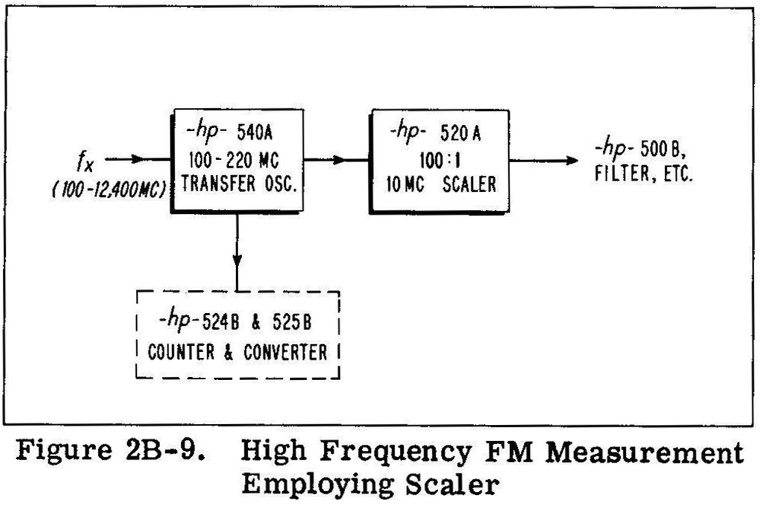
The fundamental component of the modulation is 60 cps which is combined with a large amount of second harmonic. If desired, an accurate measurement of each of the components could be made by applying the waveform to an harmonic wave analyzer (Figure 2B-8). If deviation larger than 100 KC peak-to-peak are encountered, the -hp- 520A 100:1 sealer can be connected ahead of the
____________________
1. Dexter Hartke, “A Simple Precision System for Measuring CW and Pulsed Frequencies Up to 12,400 MC”, Hewlett—Packard Journal, Vol. 6, N0. 12, August, 1955.
frequency meter (Figure 2B-9). This will allow deviations of up to 10 MC peak-to-peak to be measured.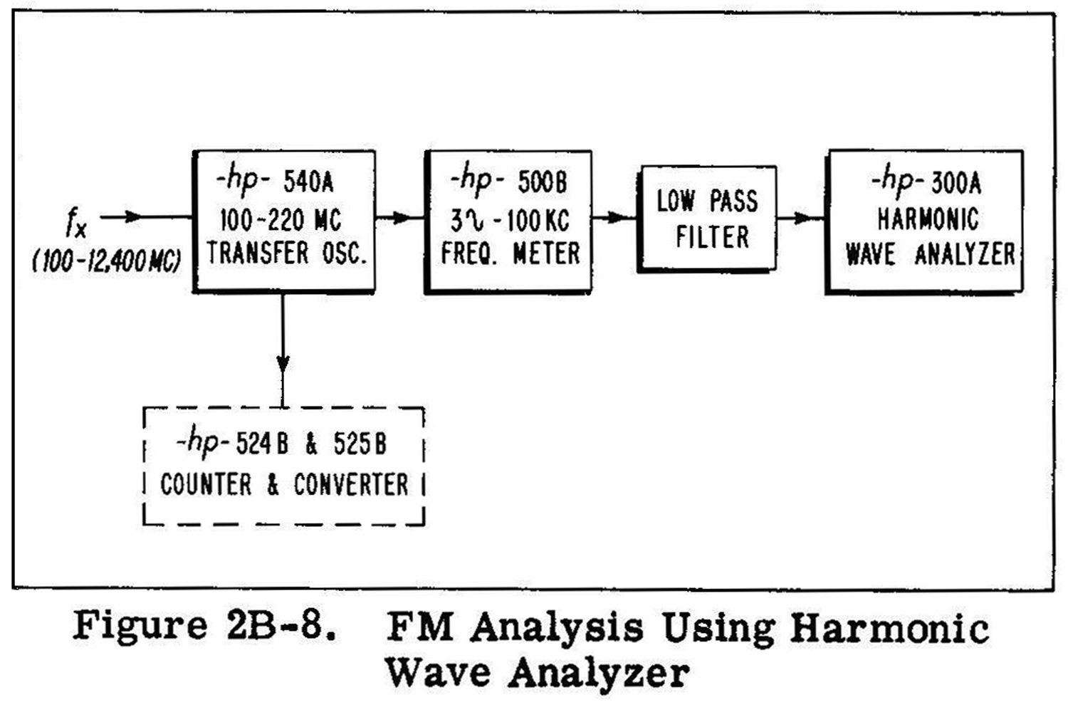
 2B-15 MEASUREMENT SET-UPS
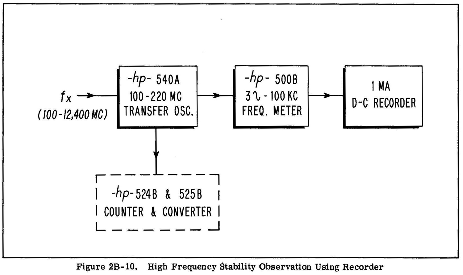
The 500B frequency meter is a versatile tool for investigating many frequency and stability phenomena. Figures 2B-7 to 2B-11 indicate how the instrument can be combined with other -hp- instruments to measure such quantities as peak-to-peak f-m deviation, components of f-m modulation, stability, and driving voltage recorders.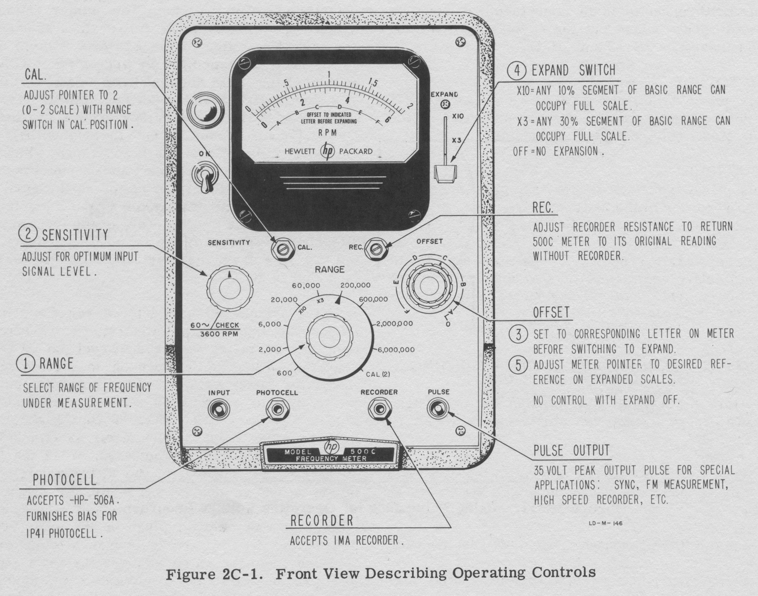
 SECTION IIC
500C OPERATING INSTRUCTIONS
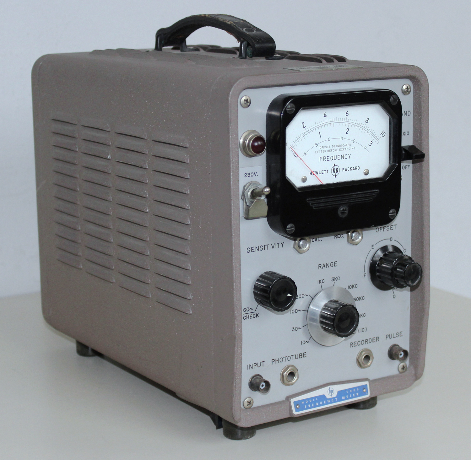
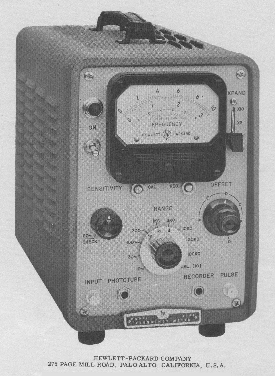
2C-1 CONTROLS AND TERMINALS
SENSITIVITY
This control, normally in the maximum position, is used to decrease the sensitivity of the input amplifier to eliminate errors resulting from spurious modulation of the desired signal.
3600 RPM CHECK
This witch position on the SENSITIVITY CONTROL places the line frequency into the input circuit. With the RANGE switch in the appropriate position (usually 6000) and the EXPAND switch OFF, the meter should indicate 3600 rpm.
RANGE
This rotary switch selects the desired range.
CAL
The CAL position of the RANGE switch checks satisfactory calibration of the constant current source in the circuit by indicating full scale on the 0-2 scale. In this position, input signals have no effect upon the meter.
CAL ADJUST
This screwdriver adjustment is used to calibrate the constant current source. See paragraph 2B-9.
EXPAND
This switch permits expansion to full scale any 10 percent (X10) or any 33 percent (X3) of the basic range in use. Use of the expanded scales is discussed in paragraph 2C-3.
INPUT
This BNC connector accepts any unknown signal from 0.2 to 150 volts rms.
PULSE
This BNC connector is an output terminal providing 35-volt peak pulses out for special applications. See paragraphs 2B-12 and 2B-13.
PHOTOTUBE
This phone-type jack furnishes bias for a 1P41 phototube permitting the direct connection of the -hp- Model 506A Optical Tachometer.
RECORDER
This phone-type jack is provided for connecting a 1 ma recorder to the instrument.
REC ADJ
This screwdriver-operated potentiometer adjusts the effective resistance of a recorder to match the instrument. The adjustment procedure is described in paragraph 2B-10.
2C-2 OPERATING PROCEDURE, COUNTING
a.Allow a period of five minutes for the instrument to reach a stable operating temperature after turning ON.
b.Turn the SENSITIVITY control to the maximum clockwise position. Place the EXPAND switch to OFF.
c.Set the RANGE switch to the 6,000,000 position.
d.Place signal under test across the INPUT connector.
e.Step the RANGE switch down from the 6,000,000 position as necessary until the meter pointer rests in the top 2/3 of the meter scale. Decrease the SENSITIVITY control and watch for a change in the reading. The reading should remain constant over a plateau of control to indicate that noise modulation is not being; measured as part of the signal under test.
It is necessary with unknown input signals to start the RANGE switch at 6,000,000 and step down, because inputs in excess of the value indicated on RANGE switch can overdrive the instrument causing erroneous readings; i.e.: 120,000 rpm will be erroneously displayed on the 60,000 range, but not on the 200,000 range and above.
2C-3 EXPANDED SCALE, GENERAL
The expanded scale feature allows increased accuracy in the measurement of changes in rpm by magnifying pointer action. The pointer action is magnified by expanding to full scale a 33 percent segment (X3 setting of the EXPAND switch) or a 10 percent segment (X10 setting of the EXPAND switch) of the range selected by the RANGE switch. The particular expanded segment represented by the meter scale is determined by the concentric OFFSET controls, which move the segment between zero and full scale of the basic range. Since the segment selection is arbitrary and the meter pointer always indicates the value of the input signal, the meter pointer will be on scale only if the selected segment includes the frequency of the input signal.
The number of rpm in the segment is indicated by the X3 or X10 on the skirt of the RANGE switch (see Figure 2C-2).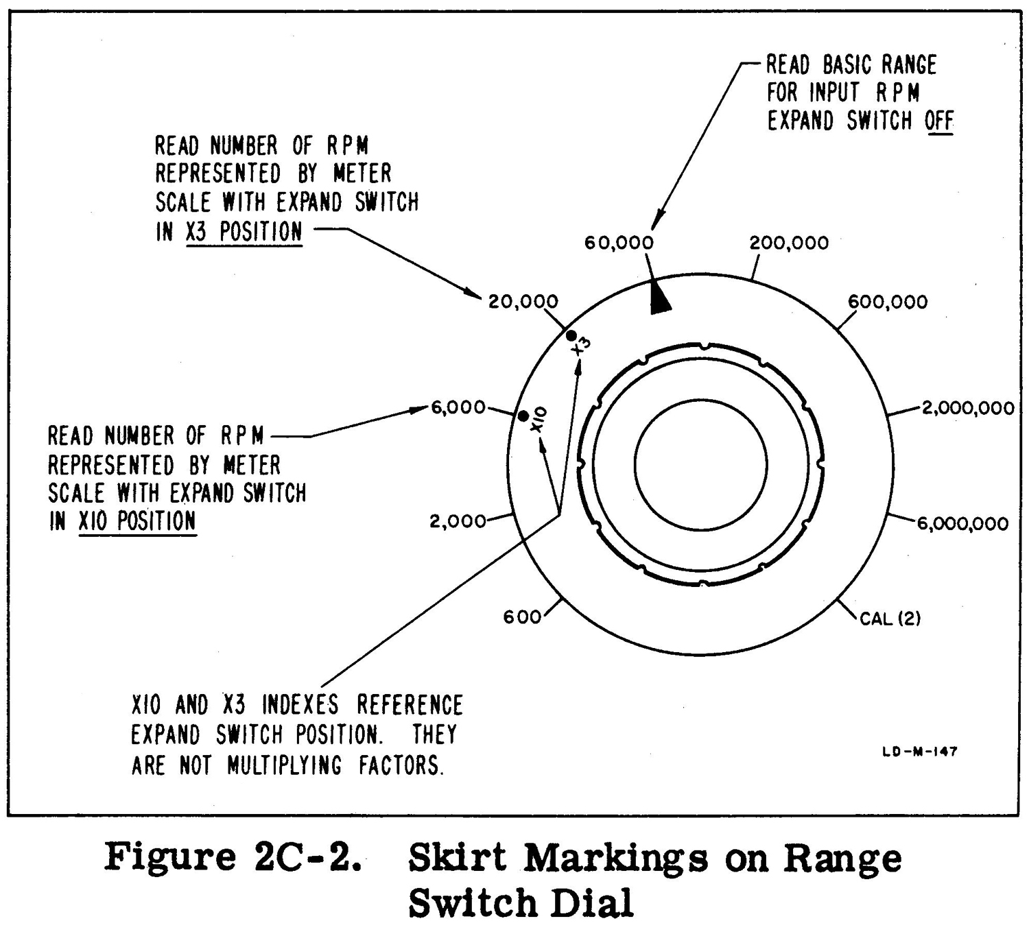 A letter system helps find the segment which includes the input signal; the letters are marked both on the meter face and around the OFFSET controls. When an unexpanded measurement is made, the meter pointer indicates a point on the letter system as well as the value of the input signal, and the coarse OFFSET control should be set near that point of the letter system before the EXPAND switch is actuated. When the EXPAND switch is actuated, the meter pointer will be on scale or not far off scale, and slight adjustment of the OFFSET controls will set the meter pointer to the desired place on the scale.
Presetting the OFFSET controls makes it easier to find the segment which includes the input signal and prevents the meter pointer from violently pinning off scale when an expanded scale is selected.
Four things must be remembered when the expanded scales are used:
1.The setting of the OFFSET controls is arbitrary! Any segment may be chosen. However, only segments which include the input signal are useful.
2.The letter system is a guide to help find the segment which includes the input signal. It is not exact.
3.The numbers on the meter scales do not indicate specific speeds because the segment can be set anywhere along the basic range. However, if the selected segment includes the input signal, the pointer indicates the relative position of the input signal within the segment. If the segment does not include the input signal, the pointer will be off scale.
4.Calibration of the meter scales is determined by the position of the pointer, the basic range selected, and the degree of expansion. For example, if the 60,000 range is expanded X3, the 0-2 scale becomes a 20,000 rpm segment of the 60,000 range. If the pointer is placed over the 1.8 marker by the OFFSET controls, and it subsequently moves to the 0.4 marker, a 14,000 rpm decrease in the input signal is indicated.
The following paragraph describes the use of the expanded scale by following through a differential measurement example.
2C-4 EXAMPLE PROCEDURE
a.Connect the Model 500C to proper source; turn on the power switch and allow five minutes for the instrument to reach a stable operating temperature.
b.Make an tm expanded measurement of the input signal as described in paragraph 2C-2. Assume that the measurement is 42,000 rpm on the 60,000 range, and that ± 6000 rpm variation is to be observed. Note that the meter pointer rests between D and E on the letter system. See Figure
2C-3.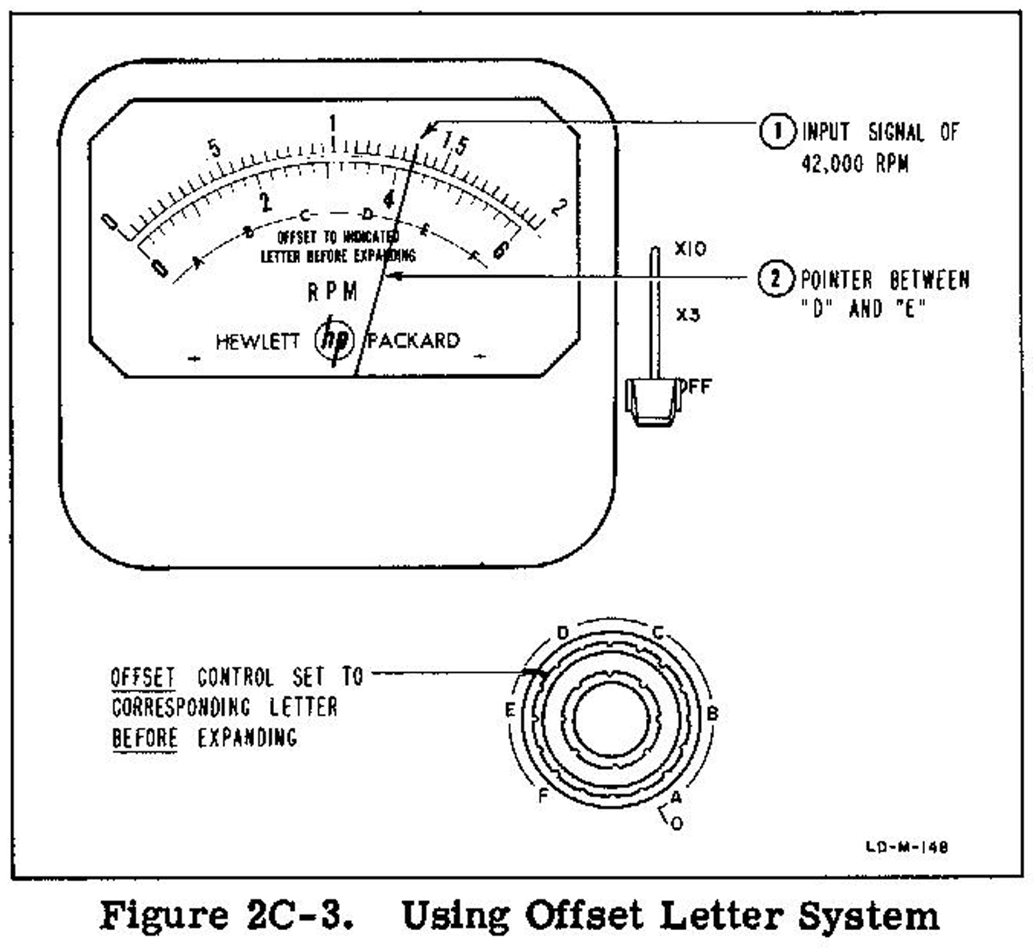 c.Adjust coarse OFFSET control to the corresponding point between D and on the letter system around the control.
d.Place EXPAND switch to X3 position. With the EXPAND switch in the X3 position, the 0-2 scale is a 20,000 rpm segment of the 60,000 range.
e. Refine OFFSET adjustment to place pointer at the desired reference. The meter pointer can be placed anywhere on the expanded scale, but to observe the ± 6000 rpm variation, the pointer must be at least 6000 rpm from either end of the scale.
Suppose the pointer is placed at “1” on the 0-2 scale. Figure 2C-4 illustrates the resulting calibration of the meter scale.
If the pointer had been placed at “0”, the “0” would have become 42,000 rpm, and the meter scale would have displayed a 20,000 rpm segment from 42,000 rpm to 62,000 rpm with the 62,000 rpm point at “2”. In this case, only the +6000 rpm variation could be observed.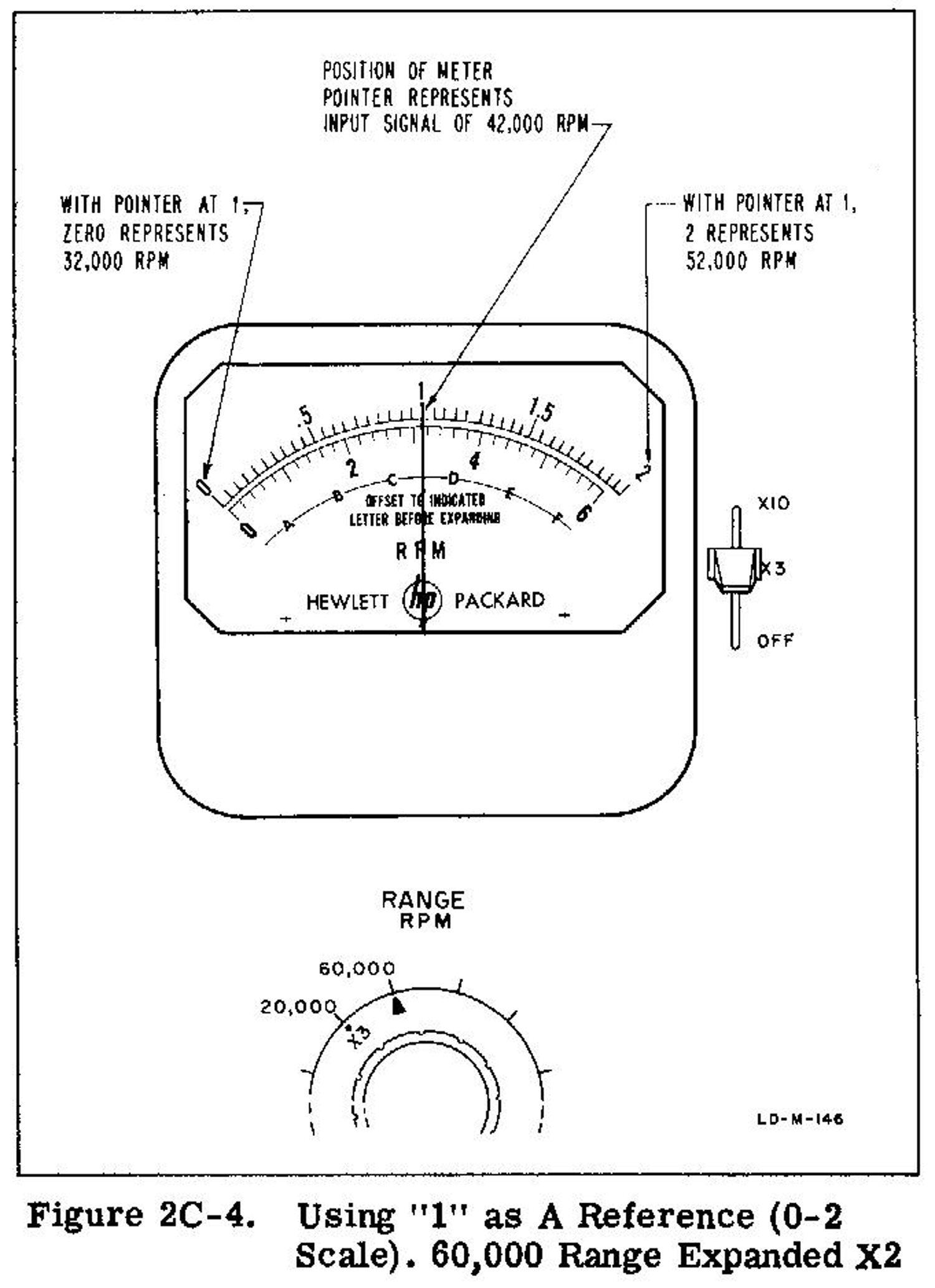 2C-4A EXAMPLE SUMMARY
Control of the meter pointer allows an arbitrary calibration of an expanded scale within a small segment of the basic range. This control establishes a reference point suitable to a particular differential or comparative measurement. In the example developed above, the expanded segment contained 20,000 rpm displayed full scale with an input frequency of 42,000 rpm. Greater pointer excursion occurs per revolution of variation than would occur using the unexpanded 60,000 scale. The greater pointer excursion allows more sensitive observation of fluctuations, variations, and drift in the input signal. It displays these changes more accurately than would have been possible on the 60,000 rpm range unexpanded.
In the example above, suppose a ± 3000 rpm variation was to be observed. X10 expansion could have been used to present an even greater pointer excursion per revolution of variation than that for X3. In the X10 case, the segment would contain only 6000 rpm (0-6 scale), and the meter pointer (42,000 rpm) would be placed at the 3.0 marker to allow the variation to be observed.
The amount of variation anticipated on the input signal governs the amount of expansion chosen. Paragraph 2B-6 discusses instrument accuracy for each measurement condition.
—————NOTE ————-
The 500B and 500C instruments are identical except for meter and range switch calibration. On the 500B, the meter and range switch are calibrated in cycles per second. On the 500C, the meter and range switch are calibrated in revolutions per minute. Thus the two instruments are operated in the same way, and identical results are obtained from identical inputs. For example, the 500B will display a 500 cps input as 500 cps; the 500C, with the same input, will display 60 × 500 or 30,000 rpm, which is equivalent to 500 cps.
The paragraphs above (2C-1 through 2C-4A), which pertain only to the 500C, parallel exactly paragraphs 2B-1 through 2B-4A, which pertain to the 500B. Section IIC is written to avoid any confusion which might arise from attempting to operate the 500C from the 500B operating instructions. However, paragraphs 2B-5 through 2B-15 will not be duplicated for the 500C. Simply remember to convert cycles per second to revolutions per minute when applying these paragraphs to the 500C. This means that the input frequency in cps multiplied by 60 will give the reading obtained on the 500C.
SECTION III
THEORY OF OPERATION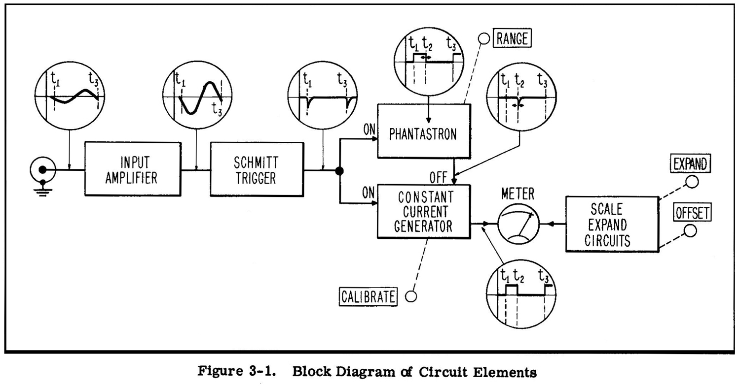 3-1 INTRODUCTORY
This section describes circuit operation for the Model 500B by discussing each element of the block diagram shown in Figure 3-1.
3-2 INPUT AMPLIFIER, V1
V1 is a conventional differential amplifier with V1A acting as a cathode follower driving the cathode of V1B. Since there is no variation in the V1B grid source (bias network consisting of R8 R9, R11), V1B acts a a grounded grid amplifier.
Bias for V1A and V1B is provided by the network R4, R8, R9, and this bias is fixed at ac ground through C3. Because V1A has no plate load it tends to conduct more current than V1B so the bias network furnishes more bias for V1A than for V1B and equalizes the plate currents in the two sections. The output signal from the input amplifier is coupled to the Schmitt Trigger through C5. 3-3 SCHMITT TRIGGER, V2
V2 is a Schmitt Trigger, conventional in all respects except in the use of C6, which permits the amplitude of the output wave leading edge to be greater than that normally encountered in the conventional circuit.
The positive going portion of the trigger output is eliminated by one-half V3, while the negative going portion is differentiated by C7 and R20 and passed through the other half V3 as a negative spike to the V4A grid.
The sensitivity of the trigger is adjusted by R12 which adjusts the no signal voltage on the V2A grid.
3-4 SWITCHING MULTIVIBRATOR, V4
V4 is a one shot cathode coupled multivibrator. In the no signal condition V4A conducts while V4B is cut off. A negative spike from the trigger V2 cuts off V4A causing the rapid switch in conduction to V4B associated with multivibrators of this type. However, V4 is not a true multivibrator because it does not return to the no signal state of its own accord. Recovery is determined by the action of the phantastron circuit, V5 – V7.
3-5 SWITCHING CONTROL CIRCUIT
As a negative trigger spike hits the V4A grid, a positive switching pulse appears on the V4A plate. This pulse is coupled to the phantastron tube V5 through C11 and C12, starting a typical Miller voltage rundown in the phantastron circuit1. At rundown start, the screen voltage on V5 rises holding the V4B grid against the diode clamp V7A, thus maintaining conduction in V4B during the rundown period. At rundown completion, the screen voltage on V5 descends cutting off V4B. The period of the rundown is fixed by the RC time constant selected by S1, RANGE switch.
Phantastron action, therefore, causes V4B to develop a current pulse during conduction which is stable in length. At the same time degenerative action of the V4 cathode resistor and the action of the clamp V7A causes the current pulse to be stable in amplitude. One such stable pulse is passed through the meter circuit for each input cycle. The meter averages the pulses it receives and presents an indication proportional to average frequency.
__________________
1. An excellent discussion of the phantastron circuit may be found in Terman, F. E. and Pettit, J. M., ELECTRONIC MEASUREMENTS, 2nd Edition, McGraw-Hill Book Co., New York, 1952.
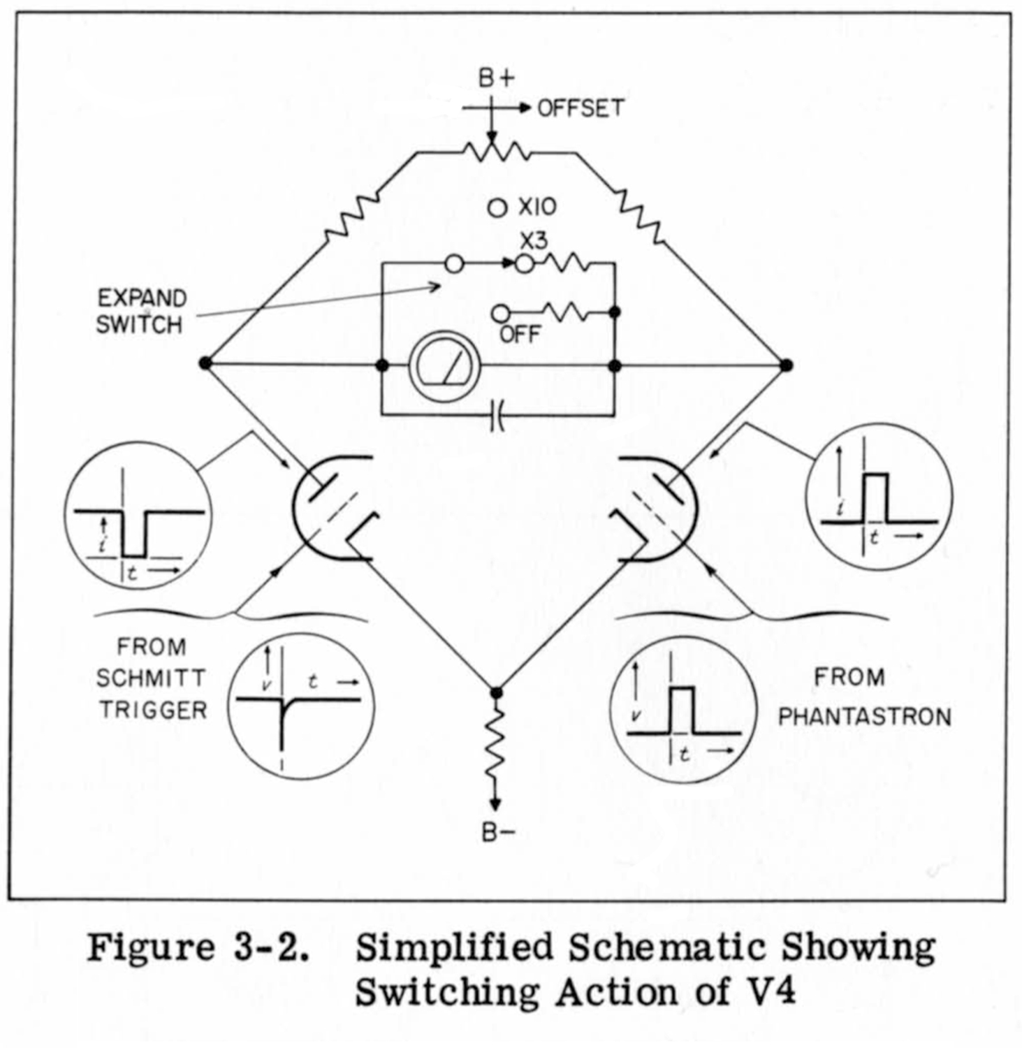 3-6 EXPANDED SCALE
When the expand switch is placed in either X3 or X10, the meter shunts, R32 and R30, are removed respectively, and the OFFSET control R24 and R25 is placed across the meter. This configuration is essentially a bridge as shown in Figure 3- 2.
The two halves of V4 conduct alternately and represent two arms of the bridge. The input frequency determines the current ratio in which the tubes conduct. The bridge is balanced for the input frequency with the OFFSET control to keep the meter pointer on scale. Resistor R27 preserves the calibration of the meter circuit over the range of OFFSET control.
3-7 CALIBRATION
When the Range switch S1 is placed in the CAL position the circuit action is as follows: The grid of V4B, the Switching Multivibrator is disconnected from the -320 volt bus and rises against the V7A clamping voltage. This allows V4B to conduct through the meter circuit, while V4A is cut off. The amount of current through V4B is then adjusted by means of R35 in its cathode circuit. The amount of current through V4B determines the amount of current flowing through the meter and the OFF position shunt of the EXPAND switch S2. This shunt consists of R31 and R32.
The meter is calibrated when the steady current through the meter circuit from V4B produces a full scale deflection (or 10) on the meter.
Adjusting R35 will produce this calibration.»
§§§
Per consultare la prima parte scrivere ”500B” su Cerca.
Foto di Claudio Profumieri, elaborazioni e ricerche di Fabio Panfili.
Per ingrandire le immagini cliccare su di esse col tasto destro del mouse e scegliere tra le opzioni.